Multiband distortion with a touch of DIY

Spoiler: skip to the end for a video where all this makes (some) sense.

As a wannabe metalhead-guitarist/bassist, I was long curious about how to get a certain gnarly bass tone, that pops up again and again in modern metal & djent. Recently, watching one of Rabea Massad’s videos, I seem to have stumbled on the answer: multiband distortion. As the name hints, it essentially consists of splitting the signal into multiple frequency bands, distorting (and optionally compressing) each independently, then recombining everything. For a bass tone, this allows keeping clean lower frequencies (avoiding muddy harmonics) but distorting higher ones — where the punch and aforementioned “gnarl” come from. 

In his video, Rabea is advertising one of Neural DSP‘s plugins, Parallax: a bass multiband distortion/compressor. Convinced by the demonstration, I grabbed the plugin’s free trial, and was blown away by the sound it got out of my 180€ Harley Benton B-650. With Parallax’ (arguably fair) 100€ price tag, however, the standard cheapskate-DIY-aficionado question came to mind: “can I do this for free?*”. Probably. This post is the answer.

* Note: I’ll be working in REAPER, my DAW of choice. Conceptualy, all that’s about to come is DAW-agnostic. The implementation details, however, absolutely aren’t.

The inspiration

Let’s start by taking a look at the VST‘s interface: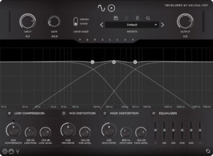

We see three filters (low-, band- and high-pass), compression and drive knobs, and an output EQ. A second tab with settings for the cabinet’s IRs is available, but we’ll ignore it for now. So far, so good: there’s a neverending supply of free distortion VSTs, and REAPER comes built-in with compressors a 3-band frequency splitter. This last little artifact, however, requires some further investigation:

All seems it place: two crossover sliders for the filter frequencies and a 2-by-6 in/out matrix (one stereo signal in, 3 out). So? Looking closer, we spot the “Param” button, indicating that this tool is a JSFX, i.e., an effect/plugin written within REAPER’s ReaScript environment. Clicking it reveals the source code for this magic (relevant bits extracted for clarity):

An ingeniously compact implementation for a low- and a high-pass filter that split the frequency bands as desired. Everything under the @sample block is executed, well… at every incoming sample, and all spl* variables refer to channels of the in/out matrix (more information on built-in scripting variables, here!). Ignoring the other variables and focusing on the structure, one can see that these are 1st-order difference equations, (i.e., differential equations represented in discrete time). As we know, 1st-order systems’ magnitudes asymptotically follow a $\pm$ 6db/oct (20db/dec) slope intersecting their pole/zero frequency. That’s exactly what we see when we push some white noise through the 3-Band Splitter, and visualize the low-frequency band’s output:

The observant will notice that on Parallax’ UI above, the filters have a -12db/oct (i.e. -40db/dec) slope — i.e., they’re 2nd-order filters. While this seems irrelevant, it turns out, the sharper crossover between bands has an influence in tone: less distortion “bleeds” into lower frequencies, which is desired. The problem is, REAPER has no such band-splitter available. What now?

Search filters on filter search

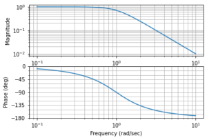
Ok, we need a steeper filter. REAPER and its aforementioned JSFX/ReaScript environment seem to offer the appropriate tool to implement one, and my memory (reinforced by some Googlin’) pointed me to the well-known Butterworth filters — a classic collection of linear IIR filters*. With the aid of the Python Control Systems Library we can take a look at a 2nd-order Butterworth low-pass’ frequency response:

$$ \begin{split} H_2(s) = \frac{ \displaystyle \omega_c^2 }{ \displaystyle s^2 + \xi \omega_c s + \omega_c^2 } \quad \xi = -2 cos( \frac { 3\pi }{ 4 } ) \approx 1.414214 \end{split} $$

Lovely: the desired attenuation after our cutoff frequency, $\omega_c = 1$ rad/s. A high-pass filter with the same attenuation — for isolating the high-frequency band — can also be obtained from the same $B_n(s)$, $n=2$ Butterworth polinomial, as 

$$ \begin{split}
G_2(s) = \frac{\displaystyle ( \frac{s}{\omega_c} )^2} { B_2(s) } = \frac{\displaystyle s^2}{ \displaystyle s^2 + \xi \omega_c s + \omega_c^2 }
\end{split}$$

Now, the next question is: how to turn these plushy s-domain continuous transfer functions into difference equations we can code with JSFX? The answer is: discretization.

* There are pros- and cons- of using either IIR or FIR filters in audio processing — in particular regarding phase-distortion — but this discussion is outside the scope of this short ramble  and of my knowledge. I’ll be sticking to IIRs here, as they’re easier to parameterize and implement.

A waveform is worth a thousand samples

The art of bringing a continuous-time system into a discrete-time domain is an endless rabbit-hole. However, there’s no need to go into the psychodelic details of the z-transform and the unit-circle; it’s enough to know that there are a few straightfoward operations that we can do to achieve this goal. Due to its stability and mapping characteristics, we’ll be using the Bilinear Transform, which does this magical conversion by mapping

$$ \begin{split} z \leftarrow k \frac{ \displaystyle z – 1 }{ \displaystyle z + 1} \quad k = 2 f_s \end{split} $$

where $f_s$ is our discrete system’s sample rate (e.g. 44.1kHz or 48kHz in audio-processing) and $z$ is the discrete  sample shifting operator. If we pluck that into our $H_2(s)$ definition above and work through the algebra (oh god my brain absolutely was not used to this anymore) we get

$$ H_2(z) =
\frac
{\displaystyle
\omega_c^2 z^2 + 2 \omega_c^2 z + \omega_c^2
}
{\displaystyle
(k^2 – \xi\omega_ck + \omega_c^2)z^2 + (2\omega_c^2 – 2k^2)z + (k^2 + \xi\omega_ck + \omega_c^2)
} $$

We can rewrite these scribbles by conveniently hiding all the noise behind $a_0, a_1, …, b_0, b_1, …$ coefficients; also, $H_2(z)$, as much as $H_2(s)$, represents the relationship (i.e., the “transfer”) between input and output signals, i.e., $H_2(z) = \frac{Y(z)}{U(z)}$. Let’s rewrite this once more, 

$$ H_2(z) = \frac{Y(z)}{U(z)} =
\frac {\displaystyle b_2 z^2 + b_1 z + a_0 }
{\displaystyle a_2 z^2 + a_1 z + a_0 }
$$

As a last sanity check, let’s pluck this into JupyterLab, defining a filter with a 100Hz cutoff:

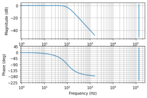
All good! Rearranging $H_2(z)$, and remembering that $z$ is a time/sample-shift operator, we can finally write our difference equation, 

$$\begin{split}
a_2 Y[n+2] + a_1 Y[n+1] + a_0 Y[n] = b_2 U[n+2] + b_1 U[n+1] + b_0 U[n] \\
a_2 Y[n] + a_1 Y[n-1] + a_0Y[n-2] = b_2 U[n] + b_1 U[n-1] + b_0 U[n-2]\\
Y[n] = \frac{\displaystyle b_2 U[n] + b_1 U[n-1] + b_0 U[n-2] – a_1 Y[n-1] – a_0 Y[n-2] }{ a_2 }
\end{split}$$

Notice that $z$ is a positive shift ($n \rightarrow n + 1$, i.e., “into the future”), which we cannot phisically do; thus, the whole difference equation is shifted bacwards, i.e., multiplied by $\frac{z^{-2}}{z^{-2}}$; presto! This whole process is then repeated for the high-pass $G_2(s)$, but I’ll spare you the pain. 

JesuSonic* has returned

* Yes, that’s unironically the original name of the language.

Last, but not least, let’s bring all this into a JSFX plugin. Thanks to good tutorials and documentation (as well as scavenging through other plugins’ implementations), one is able to get the basics fairly quickly. After a while, this is what I cooked-up (again, only the “relevant” bits are below, you can see the full thing on GitHub):

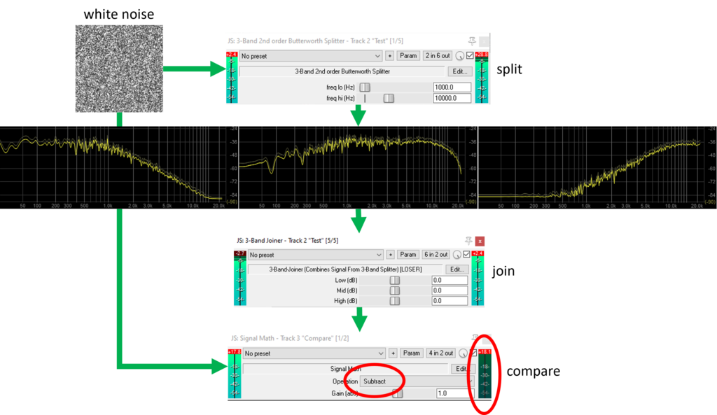
Note that 4 filters are instantiated: a low-pass pair for the stereo low frequencies, and another pair for the high frequencies. We then obtain mid=original-high-low. Worth noticing that, thanks to EEL2‘s “pseudo” OO semantics, we can use a this “pointer”, and write e.g. “flt_hi_l.iir_lp_in(s0)“, which makes stuff easier to read, IMHO. Now, does this work? Let’s push some white noise through it and find out:

As a final verification, I wrote a little “signal math” JSFX plugin (shown above) which was used to subtract the new splitter’s input from its recombined output. As expected, the output (circled in red) is zero, indicating that the original signal is correctly reconstructed. The -12dB/oct (-40dB/dec) attenuation is also clearly recognizable in the low- and high-ranges (leftmost and rightmost images, respectively). The eagle-eyed will notice, however, that the midrange doesn’t suffer the same attenuation on its sides: this is due to fact we’re computing it by subtracting the low- and high-bands from the input signal (e.g, spl2 = s0 - spl0 - spl4 in the plugin, above). This, however, is an acceptable compromise, as perfectly reconstructing the input signal is arguably more relevant.

These kids and their math; get off my lawn!

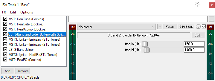
Ok, ok. Now, where’s the freaking music? Alright, below is the Parallax-copycat FX chain that I assembled:

We start standard: a tuner (d’oh!), a noise gate and a multiband compressor (whose frequency bands are controlled by the upcoming splitter). We then reach the start of the show, our “3-Band 2nd order Buterworth Splitter”: the mid- and high-range of which feed* into two instances of an guitar amp simulation**. Yes, guitar! It sounds great, and Glenn Fricker says it’s kosher, so I’m fine with it. The signals are then recombined and fed into a IR-loader***, driving a blend of a Mesa RR215 and a Hartke XL410****. Take a listen (questionable player skill and timing (in)accuracy woefully included):

* Using REAPER plugin pins (lows on 1/2, mids on 3/4 and highs on 5/6)
** The amp sim in question is the STLTones Emissary; free and really good.
*** NadIR, a free IR loader.
**** From Shif-Line’s awesome bass cab IR pack (pay-what-you-want basis).

Bringer of miracles

In the process of doing all this, I found out something cooler: unexpectedly, all of this is already done — and in a better way! 

JoepVanlier a.k.a. sai’ke offers a wide range of JSFX-based plugins on his GitHub, which can be promptly installed via ReaPack. And guess what: a 2nd-order multiband splitter is part of the fun. Go grab it — I trust his code more than mine! 

’til next time.