The Why and The What

Flying tiny drones indoors is cool, no questions asked. And stuff gets all the more interesting when you can accurately control the drone’s position in space — enabling all sort of crazy manouvers. However, using regular GPS for such applications is often a no-go: antennas may be too heavy for the drone, accuracy is above the often-desired cm range and getting GPS to work reliably indoors often requires breaking some laws of physics. For that reason, labs and research teams often turn to commercial marker-based motion capture systems. You place fancy cameras around a desired scene, fix some reflective makers on the objects you want to measure/track and some magic software gives you sub-centimeter (often sub-millimeter!) tracking accuracy. Yey. Too bad such systems are expensive. Like, way too expensive. Like, “I’d have to sell my organs on the black market for that”-expensive.

I thought: “surely someone wrote a piece of FOSS that allows me to grab some 3 or 4 webcams I have lying around and setup a poor-man’s version of such a system”. To my amazement, I was wrong (I mean, Google didn’t turn up anything, but I’d still love to run into something).  Considering that I still had to come up with some image-processing-related activity for my Masters degree, this seemed like a nice fit. So, let’s get on with it. [Disclaimer: heavy usage of OpenCV ahead.]

First things first: what are we looking for? Well, the sketch bellow sums it up: we have $N$ cameras ($C_0$, $C_1$, … $C_{n-1}$), all looking at some region of interest from different angles. When an object of interest $\{O\}$  (with some red markers) shows up in the field of view of $2 \leq k \leq N$ cameras, we can intersect the rays emanating from each of them to discover the object’s position and orientation in space.

I’m a simple camera – I see the object, I project the object

Ok, but how? Well, let’s understand how a camera works. The image below (which I shamelessly stole) represents a pinhole-camera, a simplified mathematical camera model:

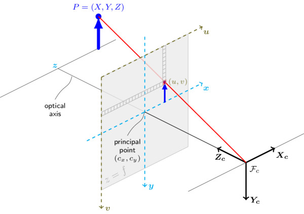
Any point $P = (X,Y,Z)$ in the scene can be represented as a pixel $\alpha = (u,v)$ via the transformation in equation (\ref{eq:projection}) below. $[R|t]$ are the rotation and translation between the camera’s frame of reference and the scene’s.

\begin{equation}\label{eq:projection} s
\begin{bmatrix}
u \\ v \\ 1
\end{bmatrix} =
\begin{bmatrix}
f_x & 0 & c_x \\
0 & f_y & c_y \\
0 & 0 & 1
\end{bmatrix}
\bigg( R
\begin{bmatrix}
X \\ Y \\ Z
\end{bmatrix}
+ t
\bigg)\end{equation}

The 3×3 matrix on the right-hand side of the equation is called the intrisic parameters matrix, and includes information about the camera’s focal distance and centering on both the x and y axes. As I’ve mentioned, the pinhole model is a (over)simplified one, which doesn’t accout for distortions introduced by the lens(es). Such distortions can be polynomially modelled, and the coefficients of such polynomial are then addressed as the distortion coefficients. No need to get into detail here, but both intrisic parameters and distortion coefficients can be obtained through OpenCV’s calibration routines. We’ll now assume all cameras are properly calibrated and lens distortion have been compensated, making the pinhole model valid.

Of blobs and vectors

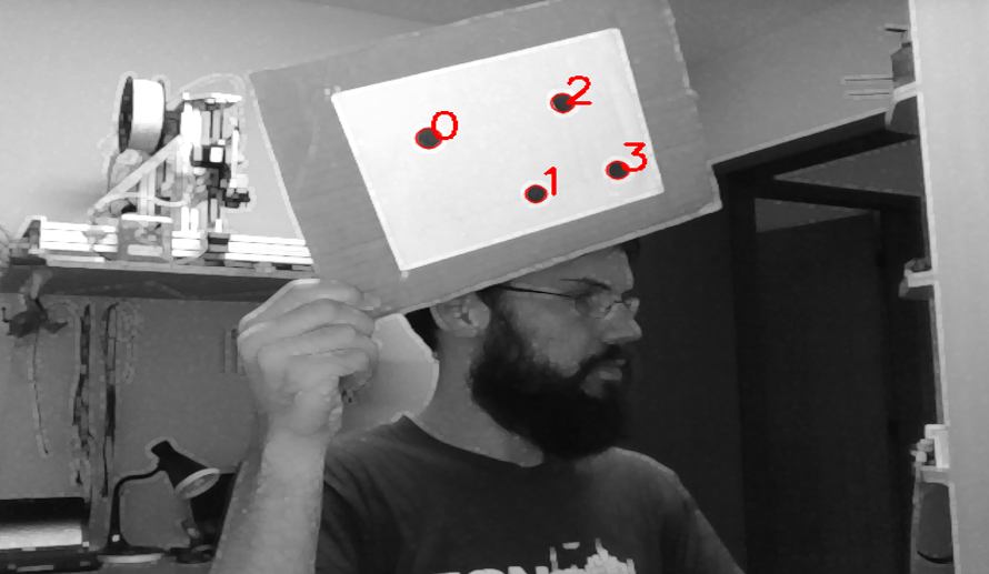
Ok, so first thing: how to find the markers — reflective or not? Well, there’s lots of room to explore and digress here, but I’m lazy and just went with OpenCV’s built-in SimpleBlobDetector (great tutorial here!). Setup and usage are straightforward and results are nice:

Ok, so the detector spits out center coordinates (in pixel space, along the $\{u,v\}$ axes) of each blob’s center point. If we want to “intersect” each view of each marker as previously sketched, then we need to compute unit vectors that emanate from each camera’s optic center $\mathcal{F}_c$ through each blob’s center. Lets assume a point $p = (x,y,z)$ – e.g., the marker – already in camera’s coordinates. Since the projective relationship in equation (\ref{eq:projection}) loses depht information, we’ll rewrite the point in its homogenous form $p_h = (x/z,  y/z, 1)$. We can then compute our unit vector $\hat{p}$ of interest from the blob’s center pixel $\alpha_h = (u,v,1)$ via,

$p_h = F^{-1} \alpha_h$

$\hat{p} = \frac{p_h}{|p_h|}$

F is our aforementioned intrisic parameters matrix. Implementing this is as straightforward as it looks:

Where art thou, corresponding vector?

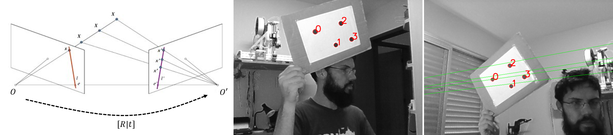
Following our system sketch up there, the next logical step is to intersect all these unit vectors we computed in each camera, for each marker. But the question that arises is: how do we know which vectors to match/intersect? — i.e., which vectors are pointing to the same marker on each camera? One convenient way of tackling this is exploring epipolar geometry (thanks for the inspiration, Chung J. et al). Simply put, knowing the rotation and translation between two cameras – e.g., O and O’ (see image below) – allows you to map a point X as seen by O to an epiline l’ in O’. This drastically reduces the search space for the corresponding X’ — that is, the corresponding view of the same object.

There’s no need to delve into epipolar geometry — specially since I didn’t learned it in detail. OpenCV supplies satisfactory documentation and great features for this. First, I’ve used OpenCV’s stereoCalibrate within a routine that continuously checks which pairs of cameras see the calibration pattern at any given time, records that information, then later computes the fundamental and essential matrices. These which encode the $[R|t]$ relationships between cameras, as shown in the figure below. Following that, computeCorrespondEpilines get’s you parameters a, b and c for the epiline’s equation $au + bv + c = 0$. So, if the n-th camera sees marker j, and a camera $n+k, k \geq 1$ sees a set of M markers, the matching view of j is m, as given by

$\operatorname*{argmin}\limits_{m \in M} au_m+bv_m+c $

Encoding this relations yields the results shown below (step-by-step usage of the aforementioned OpenCV functions can be found in the provided stereo_calib.cpp sample – worth checking out).

Transformations between cameras

So far we have our unit vectors represented on each camera’s coordinate frame, and we are able to match the vectors “pointing” to the same marker/object on the scene. Great! Now, as a last step before computing their intersection, we need to express them all in a single coordinate frame. For simplicity, the first camera (n = 0) was chosen as the main reference for the system. So, in order to express all unit vectors in that coordinate frame, we need to know $[R_n^0|t_n^0],\text{ }\forall n$. In theory, we could concatenate all the successive transformations obtained with the stereo calibration procedure, but I’ve foud that it propagates lots of measurement errors and uncertainties. For now, since I’m using a small rig with only 4 cameras, the solution is to simultaneously show all cameras a known reference (namely, an AR marker), as show below:

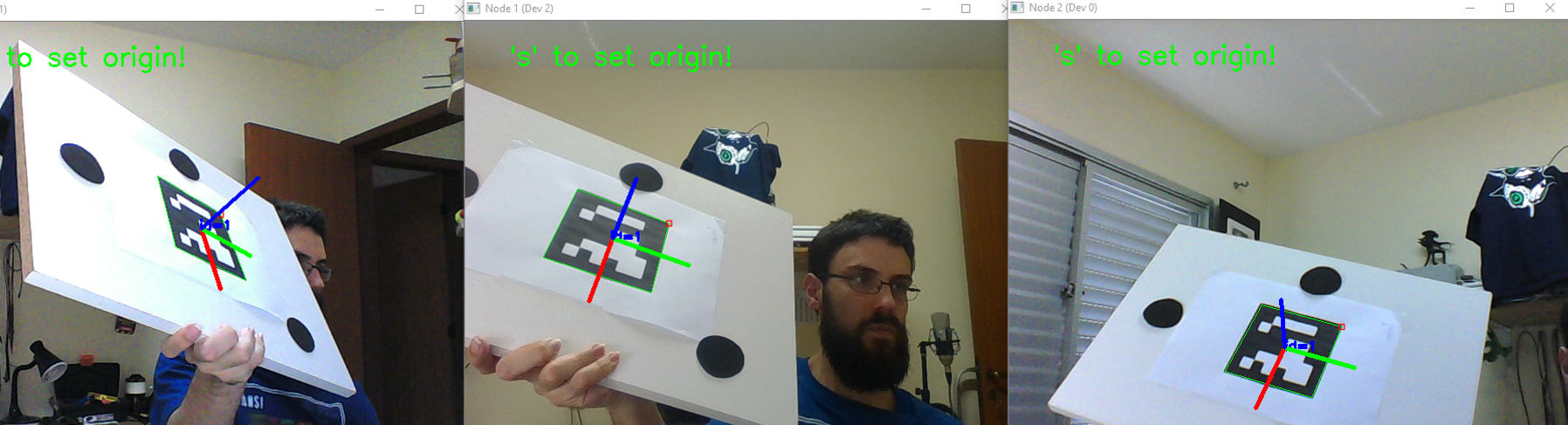
With each camera seeing the marker at the same time, we can easily compute the relationship between the 0-th camera and the n-th camera by just composing two transformations, as illustrated below:

We can then easily obtain the transformations we’re interested in:

\begin{align} t_n^0 = -R_n^0 t_n^A + t_0^A && R_n^0 = R_0^A(R_n^A)^T \end{align}

Getting to the point

Now we (finally!) have everything we need to intersect our vectors and find the position of the point(s) in the scene. I greatly recommend you take a look at this post in the Math StackExchange, since I’m piggybacking on Alberto’s detailed answer.

So, let’s assume that $k \in [2, N]$  cameras see a marker – thus we have k unit vectors to deal with. Let’s also assume from now on, that all points and vectors are being represented in the 0-th coordinate frame. Essentially, by “intersecting” the vectors, we are trying to find a point $\tilde{P}$ that is as close as possible to all the lines, minimizing the quadratic error relation given by

\begin{equation} \label{eq:reprojerr} E^2({\tilde{P}}) = \displaystyle \sum_k \bigg( ||(\tilde{P}-\mathcal{F}_{ck})||^2 – \big[ (\tilde{P} – \mathcal{F}_{ck}) \cdot \hat{p_k} \big]^2 \bigg) \end{equation}

where $\mathcal{F}_{ck}$ is the focal point of the k-th camera and $\hat{p}_k$ is the unit vector emanating from the k-th camera towards our marker of interest. This, ladies and gentlemen, is also probably the most convoluted way of writing the Pythagorean Theorem. To minimize this relationship, we look for its inflection point

$\frac{\delta E^2(\tilde{P})}{\delta \tilde{P}} = 0$

Taking the derivative of (\ref{eq:reprojerr}) and manipulating it a bit, we get

$\displaystyle \bigg[ \sum_k \big[ \hat{p_k} \cdot \hat{p_k}^T – I \big] \bigg] \cdot \tilde{P} =
\displaystyle \sum_k \big[ \hat{p_k} \cdot \hat{p_k} \big] \cdot \mathcal{F}_{ck}$

This can be represented as the matrix system $S \tilde{P} = C$. Thus our intersection point is given by $\tilde{P} = S^{+} C$, where $S^{+} = S^T(SS^T)^{-1}$ is the pseudoinverse of S.

But will it blend?

How disappointing would it be, not to have a single video after all this boring maths? There you go.

If you like looking at badly-written, hastily-put-together code, there is a GitHub page for this mess. I plan on making this a nice, GUI-based thing, but who knows when. For more info, there’s also a report in portuguese, here.

’til next time.